3.2 The self-constructed graph Mode
The aim of this applet, is to give the user an exercise tool for the well-know Dijkstra algorithm. It will be used very often for building up tables in the router. Consequently, it is important to make yourself familiar with it.
The next chapters will help you to get yourself acquainted with the functionality of the applet, the user-interaction and the analysis of the solution. But first let's introduce the algorithm itself.
The algorithm from Dijkstra (see below) is a very simple and short one. In this chapter, we take a closer look on it, with the help of the following pseudo-code. After that we will calculate explicit the solution for our graph in the tutorial mode, to get more familiar with the algorithm and the user interaction of this applet.
| 01 | ∀ v ∈ V |
| 02 | set d[v] = ∞ |
| 03 | set T = {s} |
| 04 | set d[s] = 0 |
| 05 | repeat until T ≠ V |
| 06 | ∀ v not element of T with (s, v) ∈ E |
| 07 | if d[v] > d[s] + w(s, v) |
| 08 | set d[v] = d[s] + w(s, v) |
| 09 | set p[v] = s |
| 10 | search s not element of T with d[s] minimal |
| 11 | set T = T ∪ {s} |
For a better understanding of the above used pseudo-code, we will first explain the used acronyms. The uppercase V is the set of Vertexes in the graph. The distance from the start node to an other node will be expressed by d[]. At the beginning d[] is set to infinity for each node. The uppercase T stands for a set of all nodes with the shortest path found from the start. The lowercase s is in the beginning the start node of the graph, which will automatically added to T because the d[s] = 0, which is the absolute minimum for non-negatives values. In the further execution of the algorithm, s will the newest founded shortest path node of the graph. The uppercase E is the set of all existing Edges in the graph.
At the beginning in line 1 and 2, all vertexes are set to infinity, because none of them is reachable at the beginning. In line 3 and 4 we set the start vertex. In this case node s is the start vertex and has no distance, therefore d[s] = 0. From line 5 to 11, we pass through a loop (number of nodes -1) times. It means that at each round we will find the shortest path to a node in the graph. In the first round, all reachable nodes will be added to so called "candidates", which means that they are at the moment reachable, but only temporary. It is possible to find a shorter path to one of these nodes later. This happened in line 6 to 9. After that, the algorithm searches the node which the shortest distance of all "candidates" nodes, without be a member of the set of T. The node with the minimal distance can only be a member from the "candidates", because of rest are members of set T or their distance equals infinity. After the node with the minimal distance is found, it will be added to T and assigned to the variable s, which in the next round is the initial point of finding new "candidate" nodes. After (number of nodes -1) times all nodes added to T and the routine found all shortest paths from the start node to all other nodes in the graph.
In the applet the user has to choose among three different modes. The first one, the tutorial, is an introduction to this exercise tool. It shows all the time the same graph and it can be solved easily, which the help of the next chapter. In the self-constructed graph mode the user can construct his own graph, and train the algorithm on it. You could find a precise explanation in chapter 3.2 self constructed graph mode. The last mode, the level, is the most interesting of all. Here the user starts at level 0 and has to execute the algorithm right to step up a level, if not he has to go one down. The maximum level will be 10, so after that the user proofs, that he understood the algorithm.
In the next three sub-chapters, you will find information about the special mode.
To get an easy start into the algorithm and the applet, we want to calculate an example together. Therefore we implement this tutorial. You can execute our commands directly in the applet and you will see the behavior.

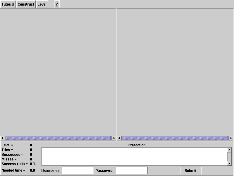
Picture 1: Start Screen of the applet
1. To start the tutorial, click on the toolbar on ![]() .
.
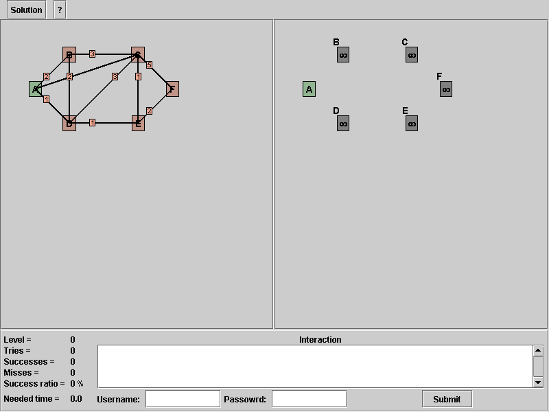
Picture 2: After you pressed the tutuorial button
What you will see is a Graph appearing in the left and nodes visible in the right. Your task now is to find the edges to all nodes, without the start node, that have all shortest paths for this graph with this start node. The algorithm is described in chapter 2, so you don't need any extra information for this now. The left stays the whole time in its original form. The right one is the place, where are you executing the algorithm.
What do you have to do first when you have to execute the algorithm?
You run the lines 1 to 4 to initialize the algorithm. But this is a very monotone work, so the applet will do it for you very time you start a mode in the applet (see picture 1). So we can concentrate on the lines 5 to 11. In the first round of the repeat clause, the variable s equals to node "A", which is our start node for this tutorial. From line 6 to 9, we are searching for the "candidate" nodes, in our case all reachable nodes are "candidate", because the distances are set by default to infinity. As a consequence, all reachable nodes from node "A" are added.
2. We have to add the edges form 'A' to 'B', 'A' to 'D' and 'A' to 'C' (How to add an edge see chapter 4.1 Add edge).
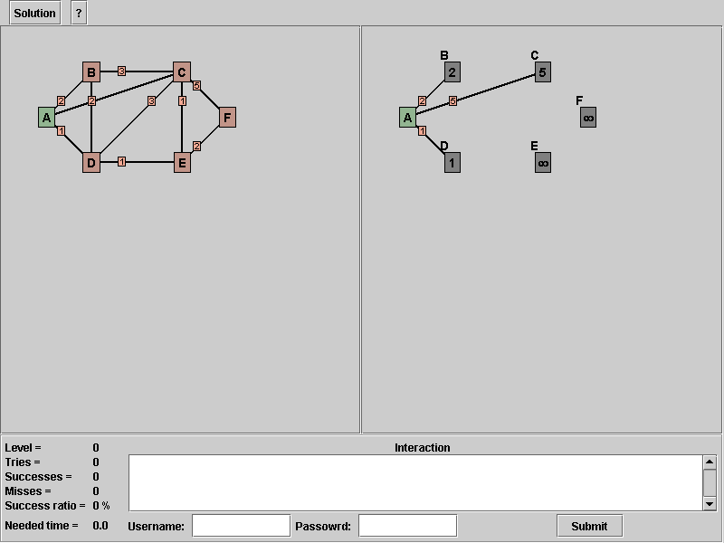
Picture 3: After adding all candidates in round one
Your solution graph should look like this, after you added the edges. Now we have to find the minimal node to the persistent set of T. We select node 'D', because it has the lowest distance by one. To have a better overview, you can select your actual 's' by right button click on the node.
3. Right button click on node 'D'.
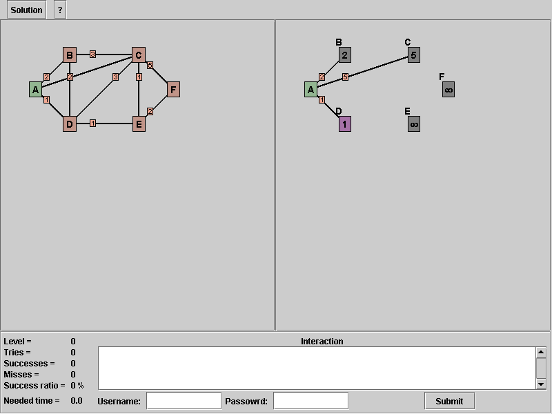
Picture 4: Finishing the first round, the next s is node d
Now the variable s shows on node 'D'. Therefore we search all new "candidates" outgoing from this node. We have four edges, that go to other nodes. These are edge "A" to "D", "B" to "D", "C" to "D" and "D" to "E". The edge from node "A" to node "D" isn't any longer of interest to us, because it is already set to the persistent solution of set T. Nevertheless, see line 6 in the pseudo-code of the algorithm. The next edge from node "B" to node "D" isn't any improvement for the distance. Node "B" is already reachable by 2 over node "A". The other two edges are candidates, because over edge from node "D" to "C" is node "C" on a shorter path reachable, compared to edge "A" to "C". And edge "D" to "E" is a new "candidate" node. Note, you have to remove the edge from node "A" to node "C", because we found a shorter path to node "C" and this edge is redundant.
4. Add the edges form "D" to "C" and "D" to "E". Then remove the edge from "A" to "C" (How to remove a edge see chapter 4.2 Remove an Edge).
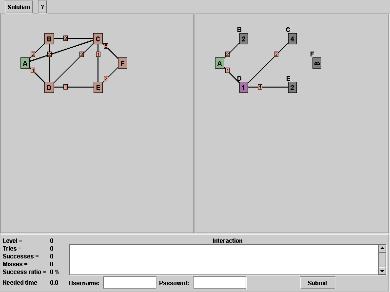
Picture 5: After updating all canidates after the second round
After you did step 4 your applet should look like the screen above. Now, we are searching the next minimum node. Our candidates are node "B", "C" and "E". The minimum distance is 2 so node "B" or "E" are the next node to select. We select node "B" as our next s.
5. Right button click on node "B".
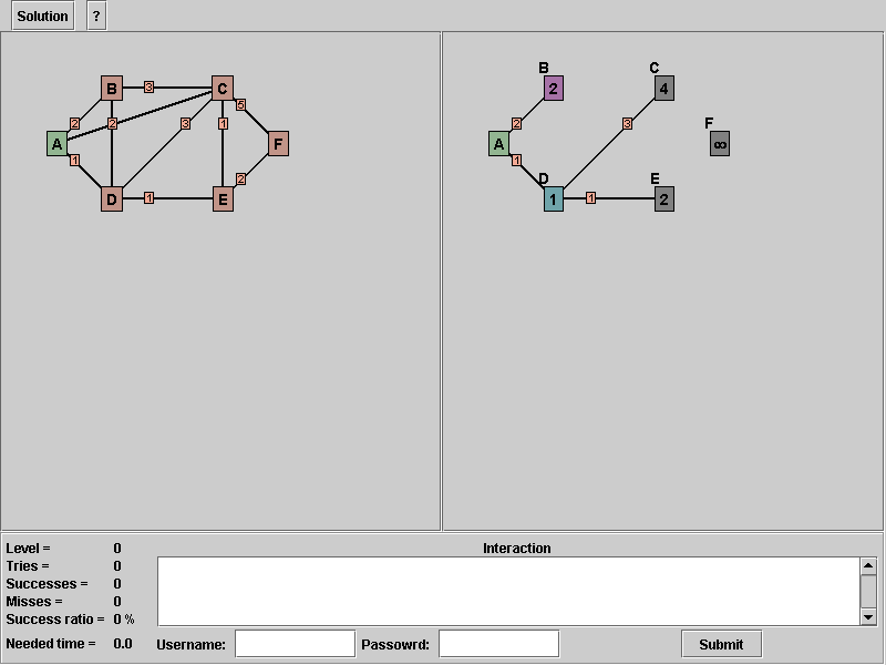
Picture 6: After selecting node "B" as the next s
Now we have all possible node colors on screen. The green stands for our start node, the purple symbolizes the actual "s" in the pseudo-code, turquoise node(s) show(s) us added nodes to the set T.
Back to our tutorial, we are at node "B", but here we can not do anything. We find no new nodes or any better path, so we go further to node "E" which has the same distance like node "B".
6. Right button click on node "E".
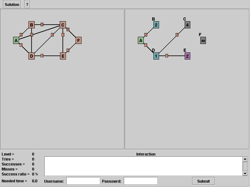
Picture 7: After selecting node "E" as the next s
Our variable "s" is now at node "E" and here we can add two edges and remove one unnecessary. We found one new node "F" and we add it to our "candidate" and we found a shorter path to node "C" over node "E". So we added the edge from node "E" to node "C" and remove the edge from node "D" to node "C".
7. Add edge from node "E" to "F".
8. Add edge from node "E" to "C".
9. Remove edge from node "D" to "C".
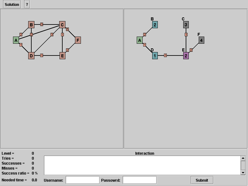
Picture 8: All changes are done from node "E"
Now there are only two unvisited nodes left, node "C" and "F". The distance to node "C" is shorter than to node "F". So we have to go to node "C".
10. Right button click on node "C".
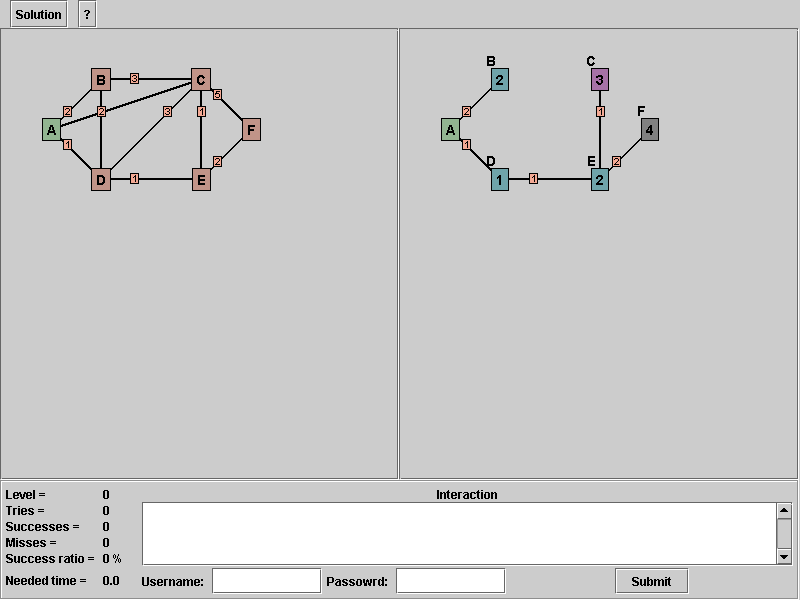
Picture 9: After selecting node "C" as the next s
At node "C" we can not do anything, so we go to node "F". Maybe we find there something new.
11. Right button click on node "F".
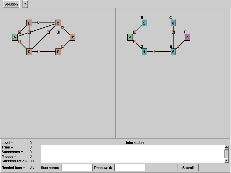
Picture 10: After selecting node "F" as the next s
Here we can not do anything, too. We reached the end of the algorithm. To visualize the correct solution we have to click on the solution button in the toolbar.
12. Click on ![]() in the toolbar.
in the toolbar.
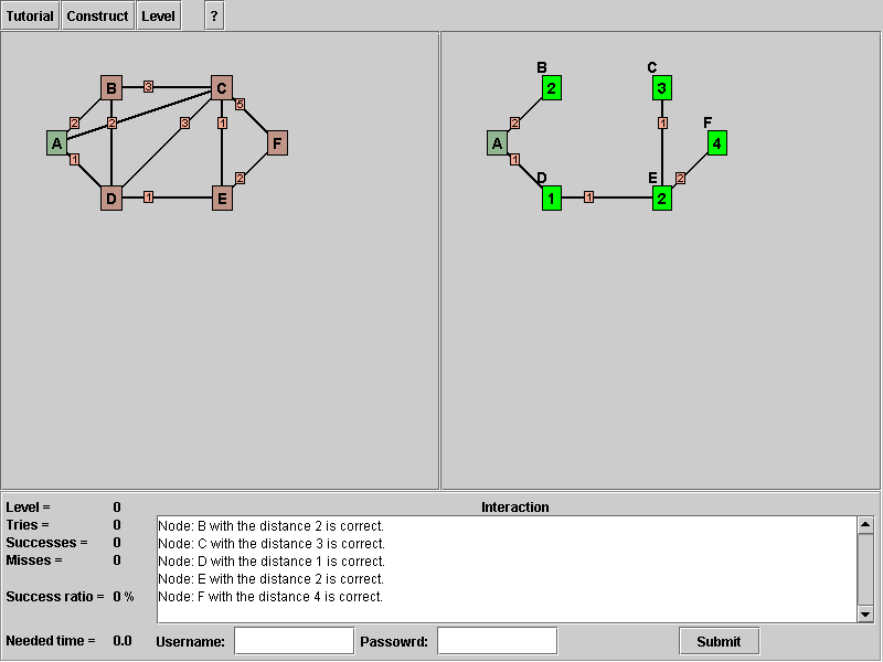
Picture 11: After pressing the solution button in the toolbar
Your see, that the nodes change their background color to green. This means you find all shortest paths from node "A" to all other nodes. To get more information about the interpretation of the solution see chapter 5
3.2 The self-constructed graph Mode back
In this mode you can easily construct your own graph and execute the algorithm on it. Afterwards, you can show the solution like in the tutorial or in the level mode. You have to be sure, that all nodes are reachable and all weights of the nodes are set to the right values. You can simply select over the drop-down-menu your favorite start node. It jumps automatically to the first added node and that is "A", but you can choose any node you want
In this mode you can exercise through ten levels. It starts with a really easy graph, much more than the one in the tutorial mode. After you go successfully through a level, you get one level up. Otherwise, when you fail you go one level down.
You need this action for building up your own graph or to add an edge to your solution graph. There are three phase for adding an edge. First you have to click with the left mouse button on a node and hold it down. Then with the depressed button you are moving to the other node of the edge and release the button on the node.
An example, you want to add an edge between the nodes "A" and "B", see below screen.

Picture 12: Two nodes, which aren't connected
To connect both nodes, you have to press the left mouse button on one of the nodes.

Picture 13: With a depressed mouse buton moving to the other node
Then you are moving the mouse cursor to the other node. Note, you have to depressed the mouse button.

Picture 14: Arrived on the other node
After you arrived on the other node you can release to the button.

Picture 15: Two connected nodes
Now, the two nodes are connected. You can set the weigth or remove the edge.
See the chapter 4.1 Add a edge. It is the same work.
You have to click the left mouse button on the panel. Note, that the new node have enough space to the others.
Just execute a right button click on an existing node.
4.5 Set the weight of a edge back
To change the weight of an edge, you have to click with the right mouse button on the weight. A dialog appears, in the field you input a new value. After that you commit by an enter or click on the button "Ok".
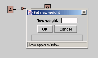
Picture 16: Change the value of a weight
4.6 Select a new start node back
When you are in the self constructed mode, you can deceided to change the start node. It hasn't to be every time node "A".
5 Analysis of the solution back
When you are calculating the minimum of a node, than the color will change to green, after you clicked the button solution.
When you are,'t calculating the minimum of a node, than the color will change into red.
if you are using to many edges in your solution, than it will be shown by encoloring the edges. Because there are not every time an unique solution, we gave an example solution. Right set edges are encolored with blue.
Wrong setting edges are encolored with red.
Missing eges are encolored with green.